With the hot potato of the x86/x64 legacy out of the way, let us now examine the new SIMD/vector unit built into NEx64T, which of course is based on those developed for those architectures (again due to the constraint of total compatibility at the assembly source level), but with a complete overhaul/redesign and several improvements/extensions.
This may sound like a small thing, but I think that the main benefit has been to have grouped the hundreds and hundreds of instructions into a few simple opcode structures/formats that in x86/x64 are, instead, dispersed in a few thousand opcodes in a pseudo-random manner.
The advantage is that it allows trivial decoding to say the least, weighing very little on both the frontend and backend of the cores. Leaving aside memory-to-memory instructions for the moment, suffice it to say that just the first two bits of an instruction are enough to identify almost all of those SIMD/vector binary (two source arguments), unary (one source argument) and nullary (no source argument) instructions, while six bits cover ternary (three source arguments), and five covers “compact” binary versions (for the most common cases).
An orthogonal ISA
This resulted in an almost completely orthogonal set of instructions, being able to operate indifferently with:
- MMX (FPU registers), SSE, AVX, AVX-512/1024 regarding fixed size registers;
- vectors and memory areas (“blocks”) with number of elements not known a priori;
- scalar (not for MMX) or “packed” data;
- 8/16/32/64-bit integer or 16/32/64/128-bit floating-point data types (the latter not for MMX);
- masks to select data lines to work on (not needed for “memory blocks.” More details later);
- possibility of resetting the data of “lines” that are not affected by the operation or copying them from the source;
- copy (“broadcast“/”splat,” in the jargon) the data read in memory to all elements;
- rounding control if operating only with registers (and not with operands in memory). Not for MMX and SSE;
- exception control always when operating only with registers. Not for MMX and SSE;
- the second source (which typically references memory) which may have a different size from the other sources and the destination. In this case the read data is converted/extended to the size of the destination (e.g., 8 FP16 data is read from the second source, which is converted to FP64 and then summed with the other source which is FP64);
- the ability to use immediate values of different sizes directly rather than referencing a memory location, saving memory accesses and possibly resulting in shorter instructions. The data is automatically replicated across all “lines” for instructions (packed or vector) that operate on multiple elements.
In a nutshell, and apart from a few exceptions that affect only the older MMX and/or SSE SIMD extensions, this means that each instruction works in any of the above contexts/modes (even combined). Take, for example:
MMADD231.H V1{K1}{Z}, V0, [RSI + RAX + 0X12345678]{1to*}
The first letter, M, specifies that it is to operate on the MMX registers (64 bits. They are mapped to those of the x87 FPU). MADD231 is the actual instruction, which multiplies the data of the second and third operands (so V0 and [RSI + RAX + 0X12345678]), then adds the results to those of V1, but subject to the K1 mask.
This means that the data of only the enabled lines (bits set to 1 in K1) will be retained, while the others (bits set to 0 in K1) will be cleared ({Z}). Since the MMX registers are 64 bits and the data type (.H) is FP16 (16-bit floating point), this means that there will be 4 data to process at a time and, therefore, 4 lines.
Interestingly, not four data are read from the third operand (the one in memory), but only one. In fact, the FP16 data taken from [RSI + RAX + 0X12345678] will be copied four times ({1to*}) to form the 64-bit “packed” block. This broadcasting/splat feature was borrowed from AVX-512, but is now available for all instructions.
This is an instruction that, as can be seen, accomplishes quite a lot of “useful work,” but above all makes use of the registers of the decrepit x87 FPU unit, which are exploited, in this case, for simultaneous processing of 4 FP16 data: something impossible for the old MMX unit, but natural for the NEx64T one, thanks to its almost complete orthogonality. Note that the instruction also makes use of a mask register (K1), which on x86/x64 was introduced and works only with AVX-512s.
For completeness I give the list and meaning of the first letter of all SIMD/vector instructions:
- M -> MMX, packed. FPU’s 64 bit registers;
- P -> SSE, packed. SIMD unit’s 128 bit registers;
- R -> SSE, scalar. SIMD unit’s registers;
- S -> AVX/AVX512-1024/Vector, scalar. SIMD unit’s registers;
- X -> AVX/AVX512-1024, packed. SIMD unit’s 128 bit registers;
- Y -> AVX/AVX512-1024, packed. SIMD unit’s 256 bit registers;
- Z -> AVX/AVX512-1024, packed. SIMD unit’s 512 bit registers;
- W -> AVX/AVX512-1024, packed. SIMD unit’s 1024 bit registers;
- V -> Vector/Block. SIMD unit’s registers (implementation-dependent size) or memory area/block (does not use registers, but memory directly. An example later).
So, and to give another example, this:
VMADD231.H V1{K1}{Z}, V0, [RSI + RAX + 0X12345678]{1to*}
will be the vector version of the previous instruction. The instruction is exactly the same, with the same coding, except for a field that specifies which of the listed modes should be used.
Here comes the new: the vectors!
It is precisely the vector version that represents the biggest change from x86/x64, which remain tied to the classical SIMD paradigm and, therefore, can handle operations on data whose size is fixed/predetermined (with a maximum represented by the size of the SIMD registers).
This means that the number of elements that can be processed simultaneously is dictated primarily by how many computational units can work on the data available in the registers involved in the operation, and secondarily by how many of these instructions can be executed at the same time in the processor pipeline.
Maximizing performance in a SIMD architecture therefore requires writing ad hoc subprograms for the specific microarchitecture. Thus potentially as many versions of the same subprogram will be needed as there are (very) different microarchitectures.
Conversely, in a vector architecture, one does not know a priori how many elements can be worked on simultaneously in a vector register, but this information is available at runtime, and only one copy of the subprogram is needed (let me simplify the discussion so as not to burden it too much) to perform the given task.
An example: daxpy – AVX-512
An example will be useful to better understand the differences between the two paradigms, having recourse to the famous daxpy routine found in the BLAS library (the de facto standard for certain types of algebraic calculations, ranging from vectors to matrices. Used in several areas, especially scientific and massive calculations), starting with the AVX-512 implementation:
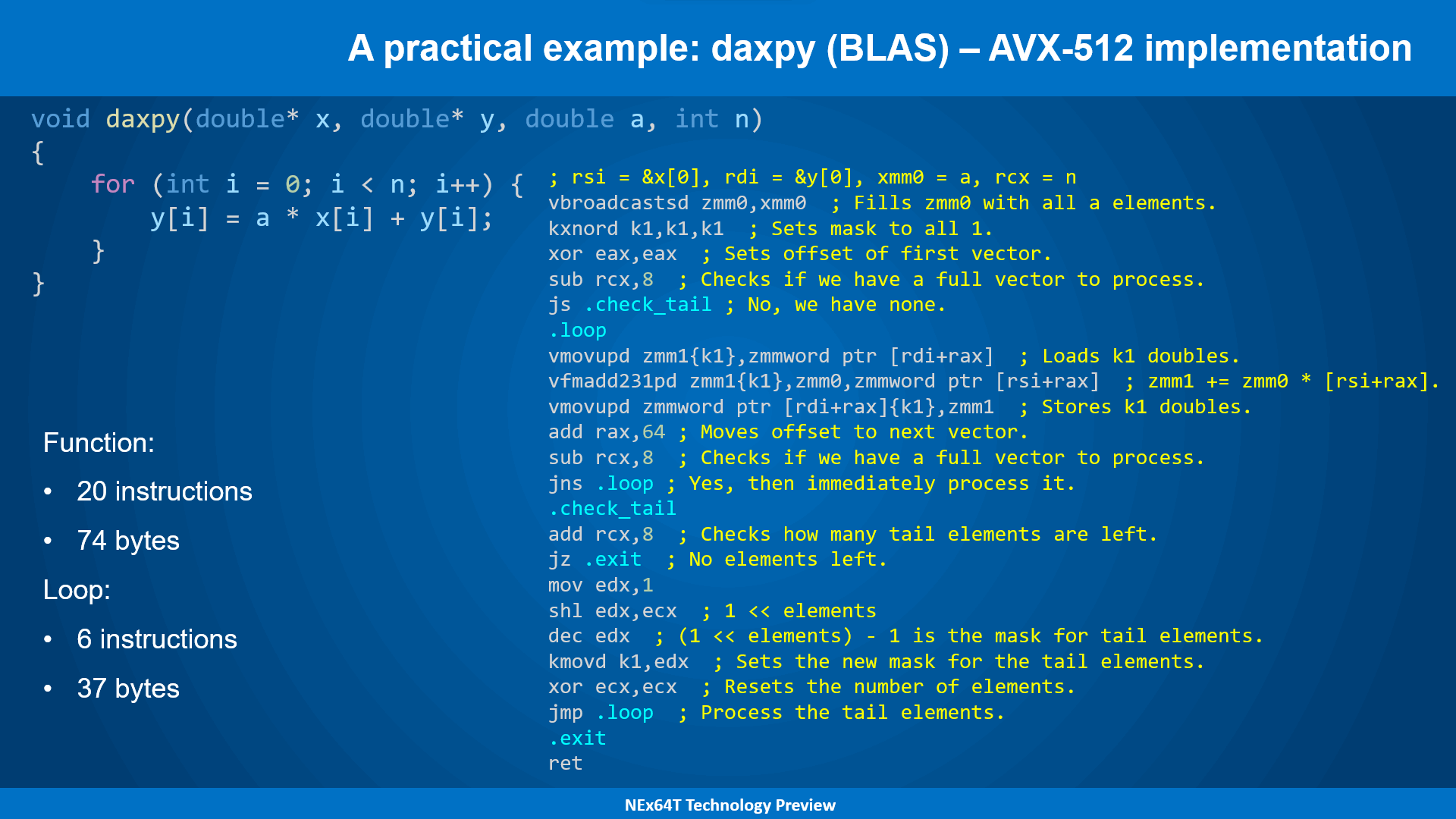
The “core” (loop) of the assembly code is quite simple and reflects, in turn, the simplicity of the function of which a C version has been reported: just 6 instructions are enough to grind out 8 iterations of the for loop at a time (AVX-512 has 512-bit SIMD registers which, therefore, can hold 8 double-precision floating-point values AKA FP64).
The complication lies elsewhere, namely in the code that takes care of initializing some stuff and doing some checking before entering the main loop (marked by the .loop label). To simplify, the concept is that AVX-512 is run at full speed, processing 8 FP64 data at a time, as long as it is possible.
Only at the end, when the vectors may contain less than 8 elements (or none at all), checks must be made and, eventually, the loop be run again for one last time, but selecting only the remaining elements (by appropriately setting the K1 mask, whose bits at 1 indicate which of them are involved in the processing).
In fact, it is the initialization and “closing” code (for the “tail” of the vectors) that requires the largest number of instructions for the purpose (as many as 14 for this alone!): far more than for the main loop (only 6, as already mentioned).
In the end, it is not even that bad, because the most important part is the main loop, precisely, which is in charge of grinding so many numbers, and objectively doing it in only six instructions is a respectable achievement.
The problem is that this implementation is fine and makes the best use (except for the “tail,” to be exact) of the resources available to the SIMD unit in the only case where the specific architecture is capable of processing at most 8 FP64 data at a time during the execution of the entire main loop (assuming, on a purely hypothetical level, that all the instructions in the loop can be executed “at the same time,” in a single clock cycle).
Obviously, the reality is quite different, and being able to process 8 data per clock cycle requires much more complex code than the above, including making use of multiple registers in which to (pre)load more data, and appropriately interleaving the instructions so as to eliminate or minimize dependencies.
This is no small amount of work, but and most likely needs to be repeated depending on the specific microarchitecture, given that each may have different requirements/constraints than another, while still being able to process theoretically always 8 data per clock cycle.
Now imagine that you are dealing with microarchitectures that allow you to compute not 8, but 16 (so two instructions) data at a time per clock cycle, and you can begin to think about what contortions are needed to try to make the most of this remarkable computational capacity.
Think, finally, of architectures that can execute even three or four of those instructions, and you already have clearly in your mind how this process is not scalable at all: it already didn’t work so well with a single instruction, but it gets enormously worse with more powerful SIMD units!
That is why in the last few years architectures have been (re)emerging powerfully that propose, instead, a return to the past, namely the vector units that had already been introduced by the ingenious engineer Seymour Cray with his very famous supercomputers.
daxpy – RISC-V
One of these, which is widely catching on, isRISC-V, an L/S (Load/Store: ex-RISC) architecture whose main advantage is that it is completely free of various licenses (apart from the trademark, which has been registered).
daxpy is implemented this way (taking advantage of the vector extension that was recently ratified, after several years of waiting):
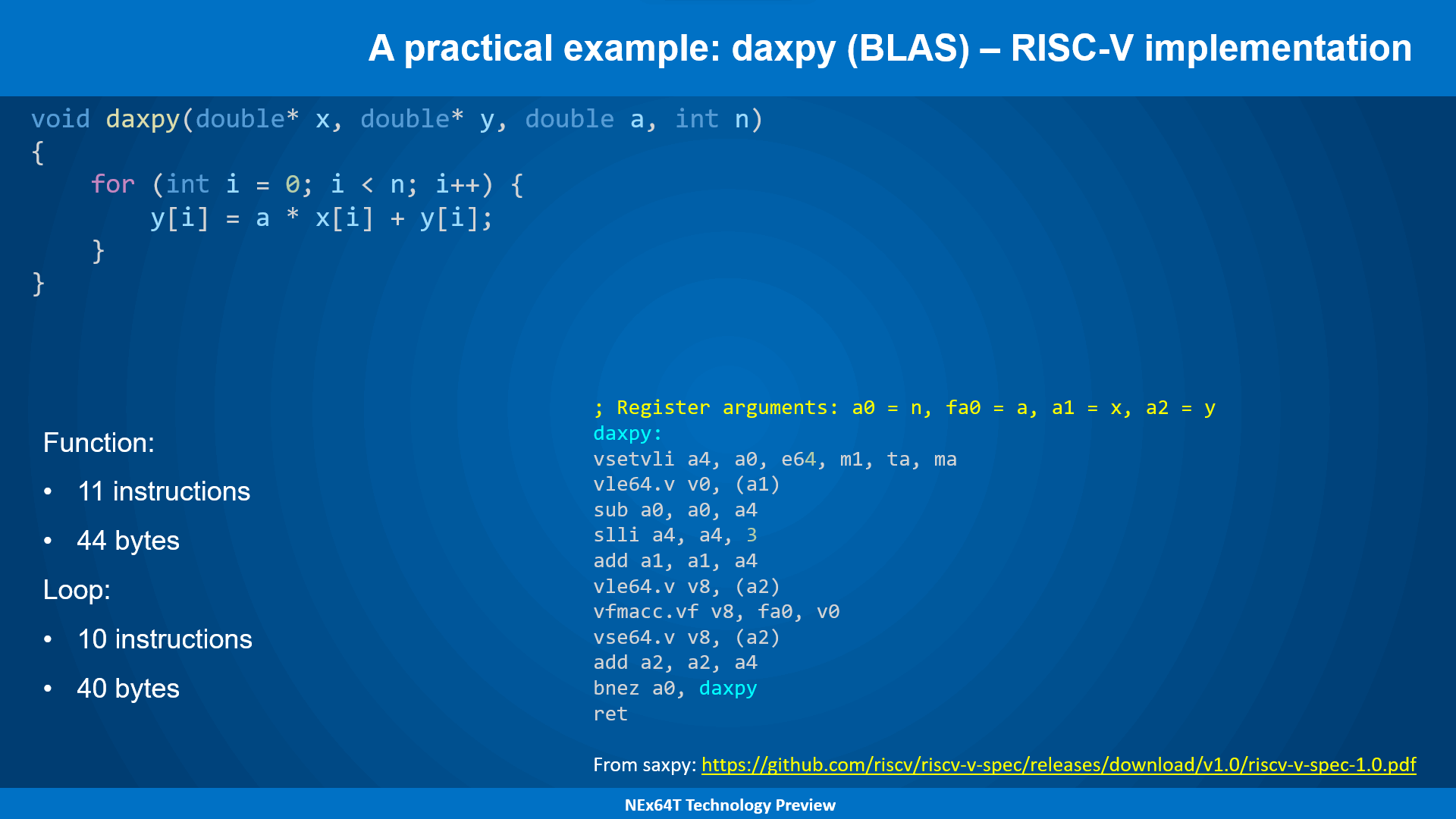
The simplicity of a vector architecture immediately jumps out at you, since there is no initialization code but, more importantly, there is no “tail” of vectors (the last elements to be processed) to be handled specially.
The main loop, however, consists of as many as 10 instructions (practically all the function instructions except the return instruction), while we have seen that there are only 6 in the case of the AVX-512 version (ignoring at the moment the initialization and “tail” management ones).
This means that AVX-512 could do better under the assumption that we are dealing with “comparable” microarchitectures capable of processing up to 8 FP64 data per single instruction (the maximum that can be handled by one instruction in this ISA).
The problem, however, is that the code also has to be changed substantially in case the microarchitecture has appreciable differences, as has been illustrated above, whereas the code of the RISC-V version does not need any modification regardless of how the particular microarchitecture on which it runs will be realized (e.g.: 16 elements that can be processed per single instruction).
daxpy – ARM/SVE
Similar considerations apply to the vector unit that ARM introduced with its 64-bit architecture (AArch64) via the SVE extension:
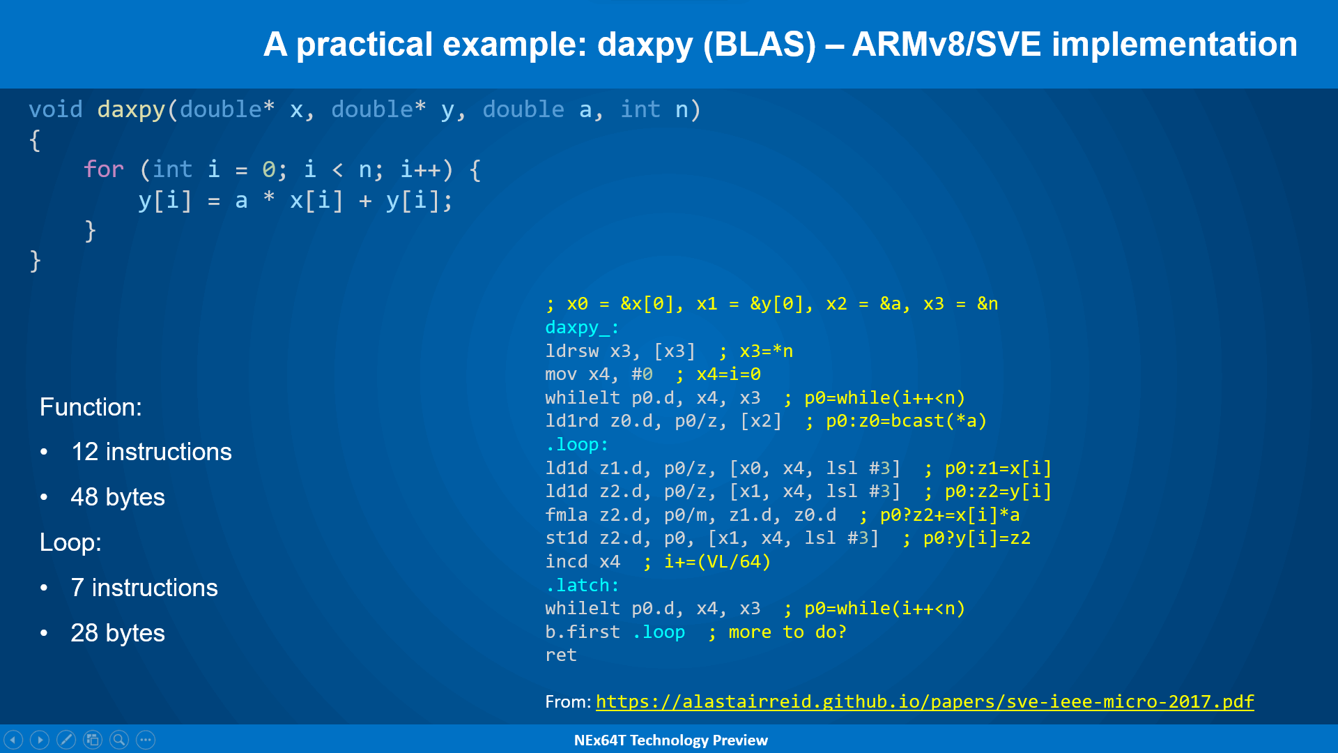
Fewer instructions are used for the main loop in this case (7, as opposed to 10 in RISC-V), due to the fact that this architecture provides more complex addressing modes (which take into account the size of the data to be accessed).
There is, however, an initialization part that precedes the loop, which is used to appropriately set a mask (p0) to properly handle the case of the “tail” of vectors as well.
Conceptually, then, ARM/SVE is a kind of “hybrid,” because it works like AVX-512 in that it uses masks to appropriately filter the elements on which to work, but like RISC-V the size of the vector registers is not known a priori (at compile time).
In any case, the goal is achieved: the processor is able to operate with an arbitrary number of elements (which depends on the specific implementation), but without any change to the code (which remains the same, for any microarchitecture).
daxpy – NExT64: base implementation
We finally come to the version for NEx64T, exposing only a basic first version, very similar to those presented so far, so as to gradually introduce its innovations and show how it is possible, as we go along, to do better:
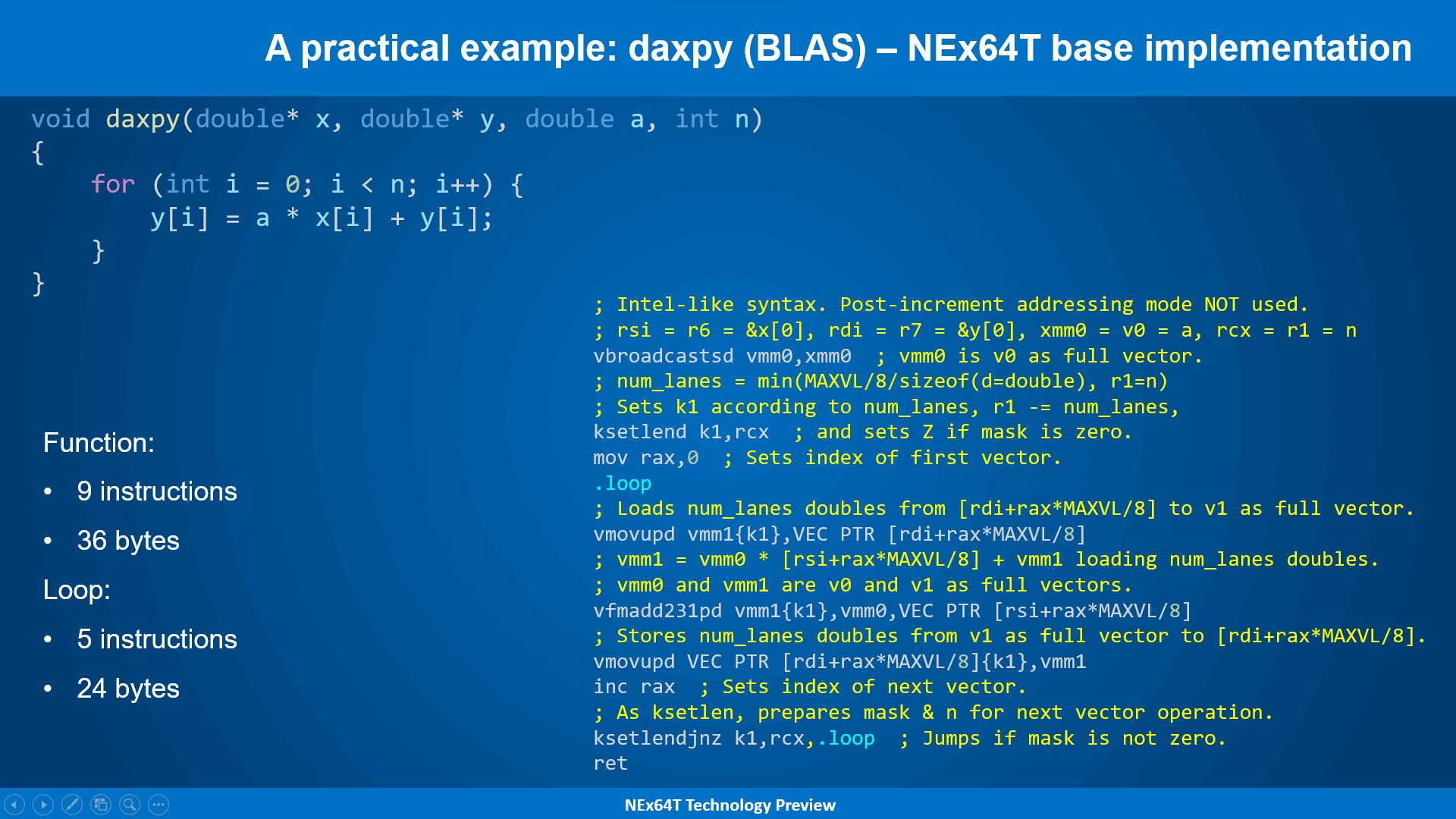
The vector extension of this new architecture is, in turn, a kind of hybrid between ARM/SVE (and AVX-512) and RISC-V. It uses, in fact, masks to select which data to operate on, but these masks are set with a single instruction that refers only to the total number of elements in the vectors (in this case it is similar to RISC-V. ARM/SVE, on the other hand, takes advantage of specific instructions to appropriately set the mask to be used, depending on particular conditions to be met).
The syntax used is similar to Intel’s, so as to make it more understandable to those accustomed to reading x86/x64 code (and AVX-512, in particular), but the comments allow it to be even clearer how the instructions work.
Meanwhile, it immediately jumps out at you that the main loop consists of only 5 instructions (as opposed to 7 in ARM/SVE and 6 in AVX-512), thanks to the use of a single instruction (ksetlendjnz) that allows you to set the new mask to be used based on the remaining elements to be processed, update how many are left (should there still be processing), and finally to jump to the beginning of the loop if there actually are still elements left.
Otherwise the code is very similar to that of AVX-512, in that the focus is on the three instructions that load the data and process it. A sign, this, that the starting base was already very good (the instructions do a lot of “useful work.” In the CISC tradition!).
Cold numbers in hand, one can see how NEx64T, albeit in a “basic” version, manages to do better than any other version, whatever the reference metrics is: from the number of instructions in the main loop (the most important, in these cases!) to the total number, from the space occupied by the main loop to the total space.
daxpy – NExT64: with post-increment
The use of a new feature, i.e., the mode with post-increment for memory addressing, allows these numbers to be lowered even further, bringing those in the main loop to only 4 instructions (but it benefits, in any case, the whole function with a general reduction in their number):
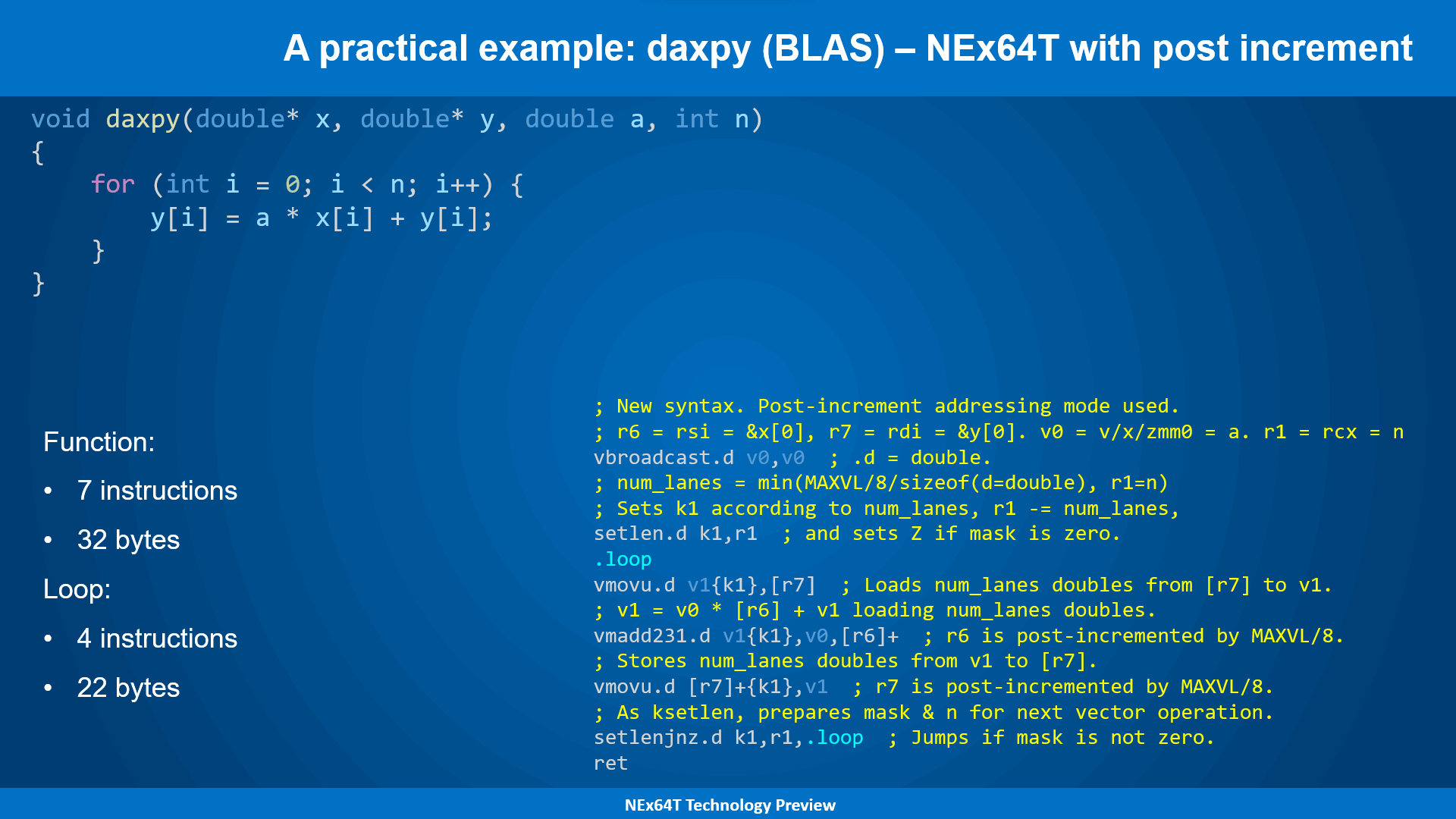
The ability to automatically advance the vector data pointer to the elements of the next group of data to be processed makes it possible to reduce the main loop to the bone, which now turns out to consist only of the data loading and processing instructions, with the only instruction (setlenjnz) remaining for checking & passing to the next block to be processed.
The initialization code is also slightly streamlined, as we no longer make use of the index that references the first element from which to start with vector data processing and, therefore, the related instruction (which sets it to zero, at the beginning).
This example is very important because it shows a fairly realistic as well as common scenario regarding the processing of vector data, in that it is the instructions that do the actual calculations that take over, with the “control” instructions playing a minimal role (the bare minimum).
daxpy – NExT64: “memory-to-memory” version
The daxpy routine allows you to show how you can take advantage of an additional NEx64T feature that allows you to minimize the main loop (which now consists of only two instructions!):
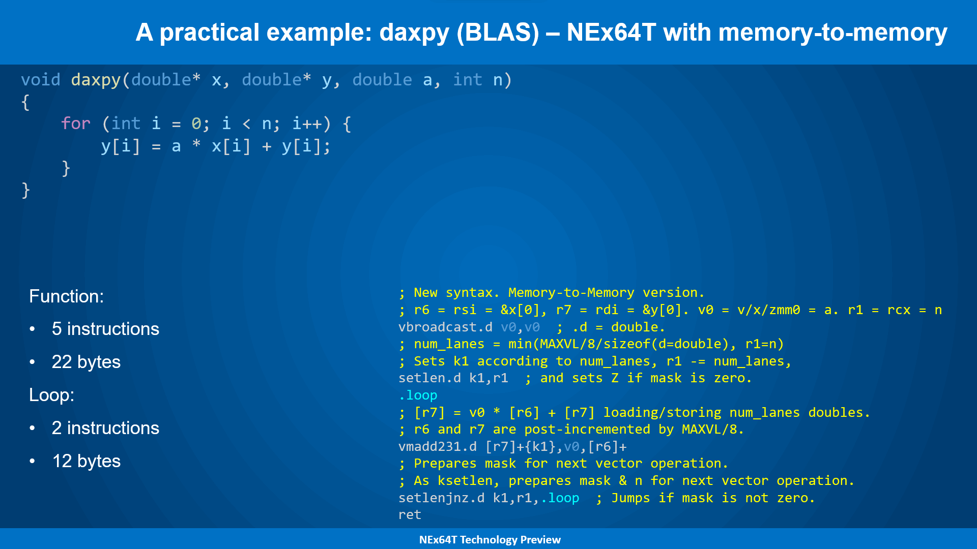
In fact, in this case, there is only one instruction that “grinds” all the data, taking charge of:
- their reading from memory;
- processing;
- writing the result to memory.
This was possible because one of the data (the multiplication coefficient) is already available in a register (v0) and, therefore, there is no need to load it from memory, reducing the number of arguments that directly reference memory to only two (the maximum possible for this new architecture).
In more common scenarios, it will be necessary to add another instruction to read (or write) the data from memory, but in any case it will be fairly easy as well as common to take advantage of being able to directly reference memory for at least two of the instruction arguments (not just vector instructions: it is also possible to do this with general-purpose ones, as discussed in previous articles).
daxpy – NExT64: “memory block” version
Again daxpy offers to introduce another innovative feature of NEx64T, which can be definitely useful in very simple scenarios like this:
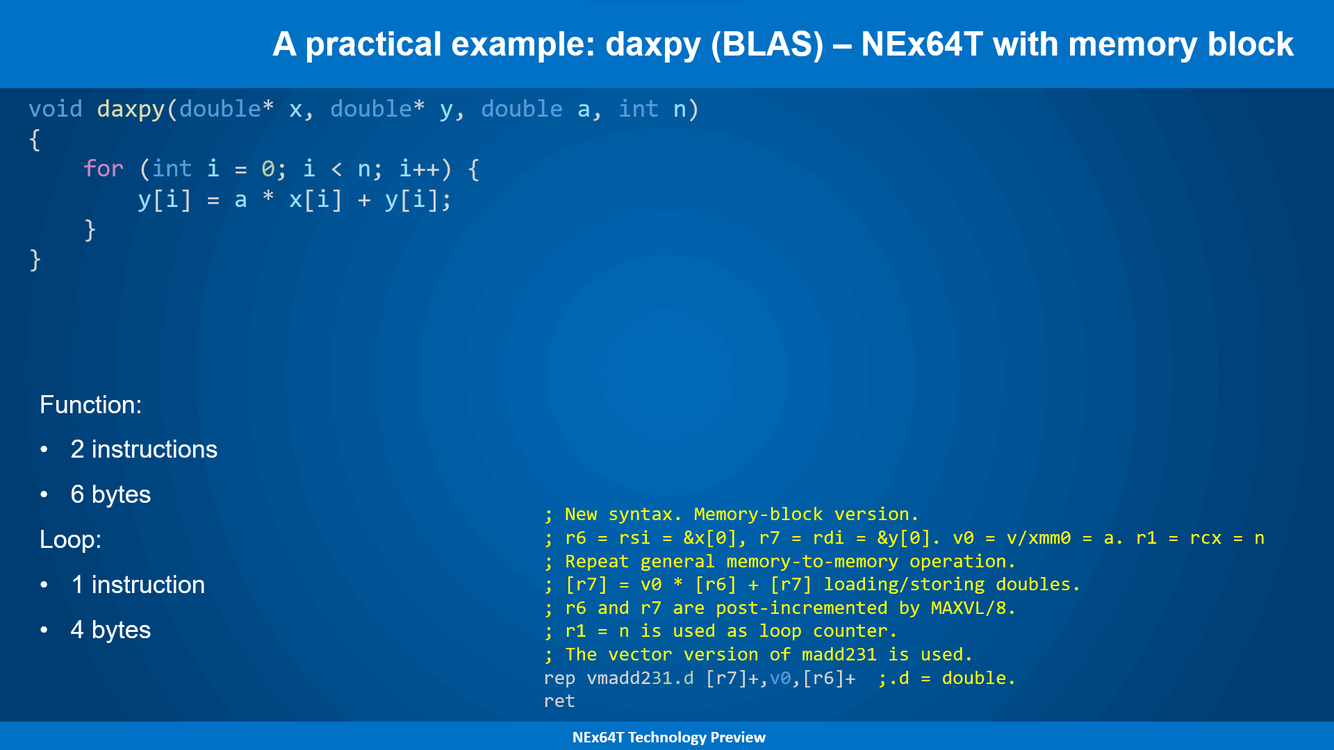
This is no joke: the code that performs all the calculations has been reduced to a single instruction, with the next one serving only to exit the function!
This was made possible by NEx64T’s ability to employ any general-purpose or vector instruction for the so-called “block” mode, which extends the concept introduced by x86/x64 with the REP prefix (which, however, could only be used on a few, very limited, instructions).
The idea is to generalize the concept of input and output of the “to-be-repeated” instruction by having data taken from any source (in memory, making use of certain addressing modes. Or from a register) for the input operands, to any destination (using the same modes).
In this case, it is sufficient to store pointers to the memory areas to be read or written in precise registers (r6 for the second source. r7 for the destination) or to specify the register in which the “scalar” data is stored (v0, in this case).
The processor will then take charge of:
- read all the data gradually;
- pass them to the “to-be-repeated” instruction;
- drawing the result from it;
- store it in the destination;
- automatically update all pointers to move to the next data (and destination);
- update the item counter until there are still some left to process.
So NEx64T revives and breathes new life into a concept considered obsolete as well as a harbinger of criticism, but one that allows for extremely efficient implementation of, yes, simple, but also quite common scenarios.
It does so, then, by extending its capabilities, thanks to the ability to specify addressing modes other than those of x86/x64 (limited to post-increment and post-decrement only), including data-stride and gather/scatter, as well as the use of registers (as seen in this example).
Finally and to close on this topic, this new architecture also revitalizes another feature first introduced by Intel more than twenty years ago, allowing the concept of repetition (and not only that!) to be exploited in a more “original and creative” way. About this, at the moment, I prefer not to talk so as not to reveal too many cards.
“Reduction” operations
Another fairly common scenario in vector calculus is what is known as data “reduction” (in jargon). This is, simply put, applying an operation by taking all the elements of a vector, starting with the first two of them, and reusing the result gradually with subsequent elements (one at a time).
The classic example is that of summing all the elements of a vector (taken from the link provided above, but corrected: the code shown there is, in fact, wrong!):
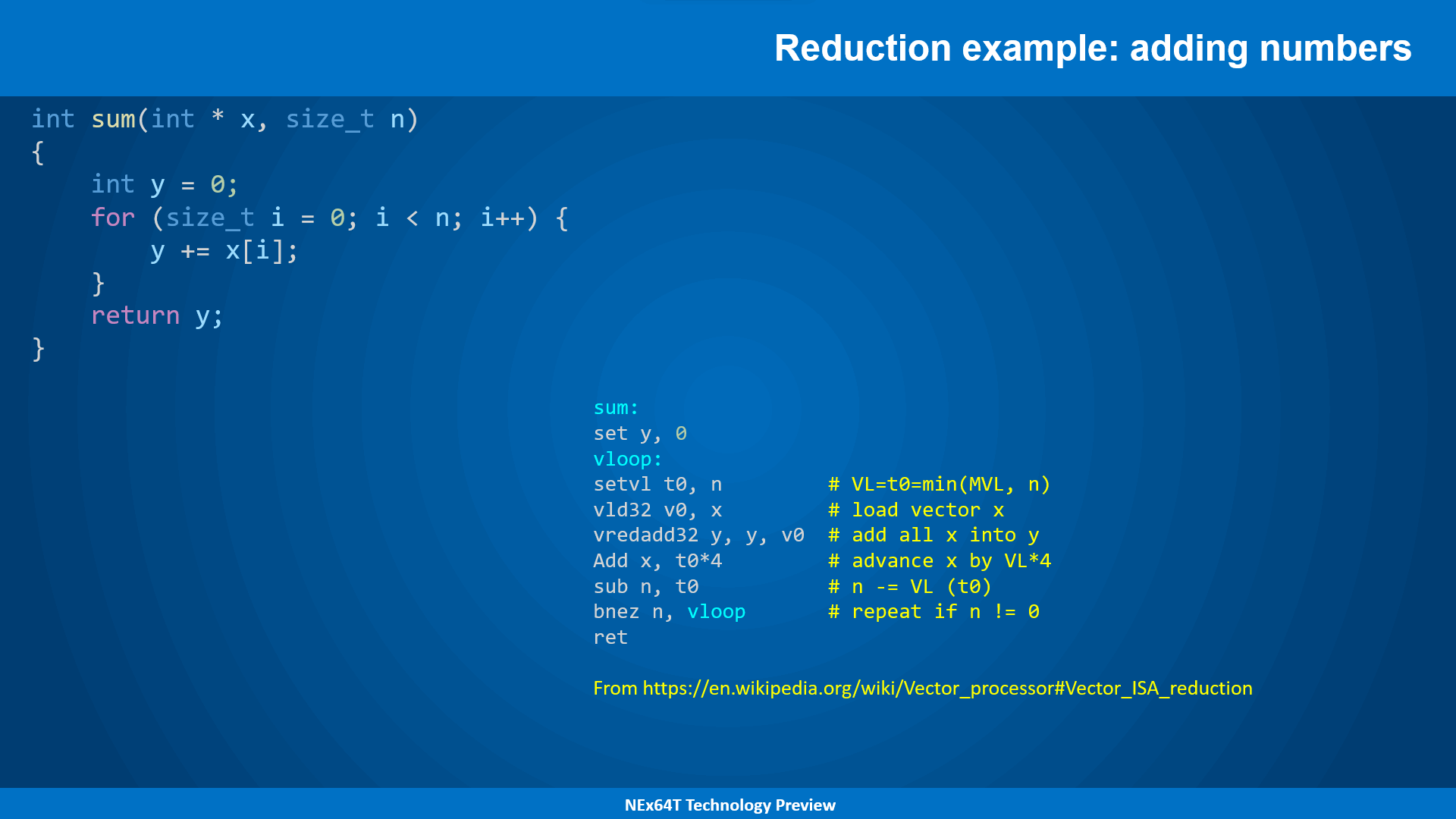
The example is, so to speak, heavily inspired by what is offered by the RISC-V architecture, but it is perfectly fine for stating the concept in a simple way, without going into details that would further lengthen the already long article.
The idea is to introduce specific instructions for these cases (vredadd32, in the example), which take care of processing the data in parallel and as much as possible, taking it from memory according to the capacity/size of the vector register, and then repeating the block of operations until all the elements have been processed.
A scenario very similar to that already presented with daxpy, in short.
Reduction with NEx64T
Needless to say, NEx64T allows one to do far better:
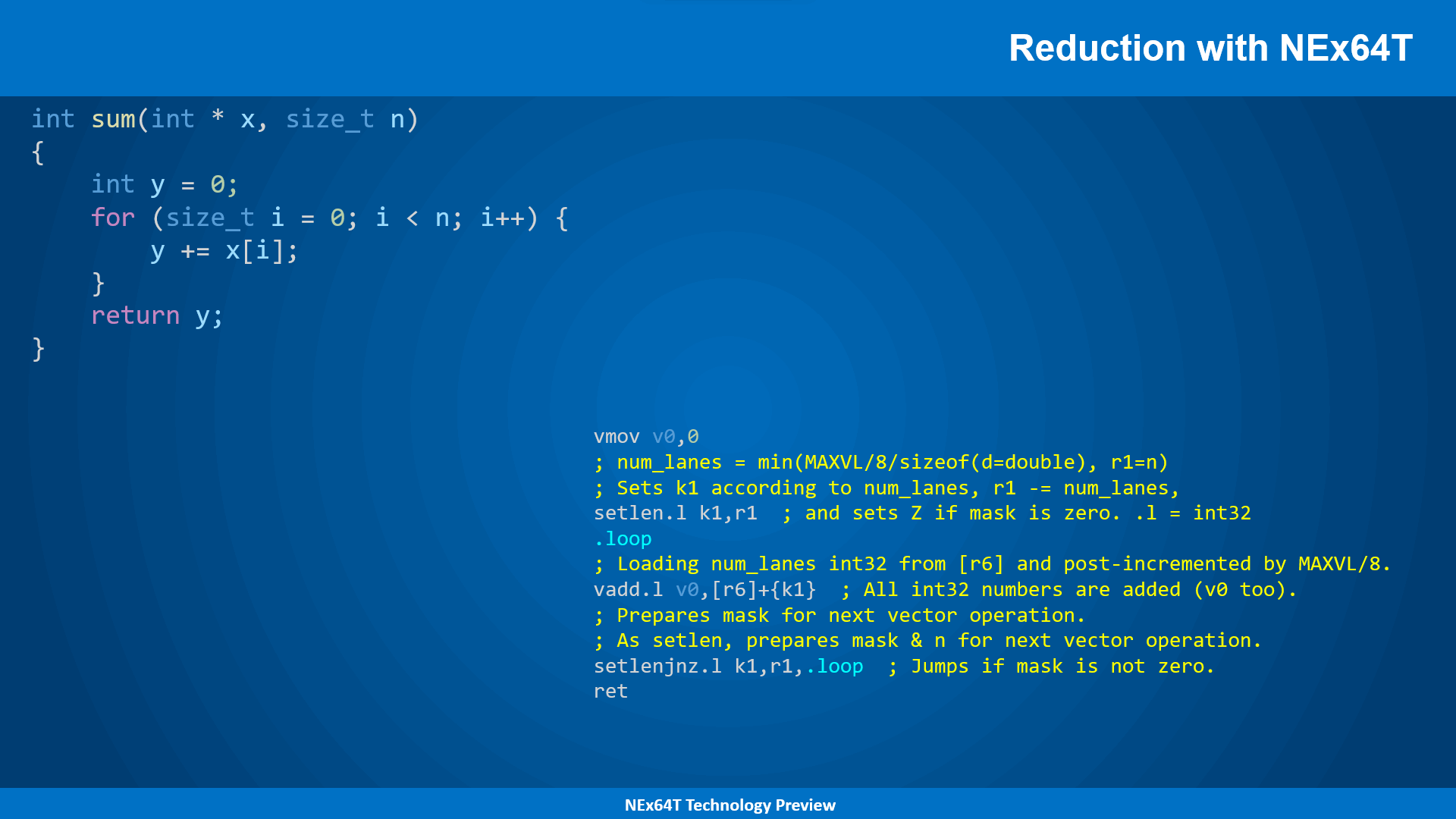
Taking advantage of the CISC tradition of being able to directly reference data in memory, the operation to reduce a portion of the vector results in… just one instruction! There is no need to add more, as the simplicity of the code is, in itself, more than sufficient to demonstrate the enormous flexibility and capability of this new architecture.
However, one particular aspect of NEx64T, which differentiates it from even better known as well as emblazoned architectures, should be emphasized: no new, special, reduction instructions need to be added to the ISA. In fact, any vector instruction is (re)usable in “reduction mode”: the backend of the processor will take charge of processing them properly to accomplish the task, completely transparently.
Another peculiarity of these instructions is that they can be “interrupted”, depending on the particular implementation adopted. If, in fact, the processor receives a very high priority interrupt signal (e.g., in a real-time system) and the backend is unable to complete the operation quickly, then the execution of the instruction will be suspended, only to be resumed once the interrupt is over.
The advantage, compared to other architectures, is that this mechanism does not require anything to be added to store the current state of the instruction, since it already stores everything needed (in register k1, in the specific example) so that it can be resumed and then continue processing.
Reduction with “memory block” version
It was a foregone conclusion, finally, that such reduction operations could be implemented by taking advantage of the “block” mode already presented, which fits absolutely perfectly for scenarios such as these:
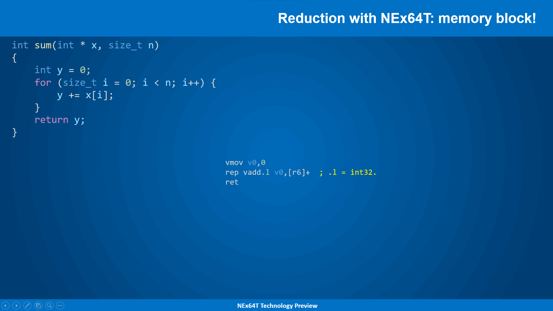
Again, nothing more needs to be added here, because the code comments for itself!
Conclusions
The time has come to close this article, which has been very long because there was quite a lot to say about SIMD/vector units, which represent one of the most important elements in modern processors (just look at how much space they occupy in terms not only of the number of instructions, but also of the silicon & transistors used to implement them).
On the other hand, these units were born to take the concept of data processing to other levels, and that is why, for the past twenty years or so, they have played a central, prominent role within processor cores, and on which much more is now invested than in “general-purpose” units.
NEx64T, as we have seen, puts a lot of meat on the fire, with an extension not only keeping up with the times, but also providing no small innovations that make it much more flexible as well as performant than the competition.
In addition to what has already been said I add on the fly some features that are important to report for completeness:
- up to 32 SIMD/vector registers are available, regardless of the execution mode (32- or 64-bit). x86 (32-bit) is, on the other hand, limited to only 8 registers (and only SSE or AVX: AVX-512 cannot be used), while x64 is limited to 16 registers with SSE and AVX, and requires AVX-512 to access all 32 registers;
- compared to AVX-512, it is possible to have up to 16 registers for masks (8 more than AVX-512), which can also come in handy in case you need to perform calculations on them;
- there is not a myriad of type conversion instructions, but only a few that are capable of converting from any one type to any other one;
- each SIMD/vector instruction can be executed conditionally (based on the flags of x86/x64).
An innovative aspect that deserves to be listed separately is that such a unit is “hybrid”. That is, it allows both SIMD instructions (thus using fixed-length registers, such as MMX/SSE/AVX/AVX-512) and vector instructions (with variable-length registers) to be mixed during execution.
The major limitation of concurrent architectures is, in fact, that they generally allow only one or the other to be used, but not both at the same time.
As we have seen, vector instructions are convenient because they make it possible to generalize the access and processing of vectors, without having to know in advance how many elements the vector unit can hold (and, therefore, process) in its registers. But it needs an initialization and finalization part that allows it to “adjust its focus” depending on how many elements are to be processed and how many are left.
In contrast, with traditional SIMD units, one already knows how many elements they can hold and process, so they can “start immediately” with processing. But they cannot handle vectors of arbitrary size, requiring special initialization and element management sections “in the tail.”
There are scenarios for which one model is optimal rather than the other, and vice versa, and this is the reason why NEx64T allows instructions of both types to be executed indifferently at the same time, providing as much flexibility as possible.
This concludes the discussion of this part of the new architecture. The next article will make a rough comparison with the competition, setting out the reasons why it makes sense to consider using this new architecture and, therefore, why it is worth investing in it.